
Cross Elasticity of Demand
The price elasticity of demand enables companies to predict changes in demand based on a rival's pricing architecture. By doing so, a company is equipped to create a more sustainable strategy, and to have an upper hand. The model is an utterly cool interpretation of pricing and the subsequent market effects - in value and volume - as it shows the interplay between four extremes. The extremes between the selected rivalry, is as simple as lowest price and highest volume and highest price and lowest volume between the rivals. The rest is pure calculations at various levels. The model is the third tier in the complete Pricing Tool.
Step 1: Do your selection
For good order, and for those who read about the Pricing Tool for the first time, you need to make a selection for your benchmark analysis.
Firstly, you make your selection (which is called product A), for then to create your benchmark product / supplier etc (named Product B). All in all, you have 33 various options in the basic model, but with options to add. You can either do the selection as a starting point, or whilst working through the various analysis.
The red and the green are simply ‘mirror’ / duplicate databases, but then facilitates both external as well as internal analysis. Say you have a 4-pak and a 6-pack for the very same brand, and wonder what yields best results for the retailers. Well, then the mirror databases will enable the understanding the best option in the short term and the longer term.

Step 2: Read the core graph
The model works perfectly well as an on/off analysis or as a max/min analysis. As a supplier, you are either on promotion or you are off the promotion, on a weekly cycled schedule. What actually happens between these extremes, is what the cross elasticity model describes the best. It is worth to mention, that it works best for ‘substitutive’ products, and when there is a dynamic effect in the market / category. A different understanding will need to be used when studying complimentary products and for non-related products, but that will not done here, for simplistic reasons.

The x-axis looks into the span in price levels, whereas the y-axis shows the volume. The play between these extremes, is however where the magic happens, and if utilized properly, tells you who to generate growth.
What do you see by first glance?
1. The extremes: Here you see 4 extremes (lowest price and highest volume, and vice versa, for two competing products).
2. The span in pricing (x-axis): The length of the lines, explains the span in pricing
3. The effect in volume (y-axis): The higher the lines, the higher the volume (read: sales)
4. The slopes of the lines explains the elasticity / dynamics between pricing and volume
We can easily see that B is larger than A, and that is also has a larger price span. We also see that the slope of B is steeper than A, telling us that it responds more to price changes. All in all, B is the market leader and is what the retailers sees. Then what about A? Let us dig deeper.
NB! You will probably ‘miss’ some analysis here, but remember that this is only one part of a bigger and more complete analysis.
Step 3: Interpret the core graph
B is the category king today, but there is also something weak with the performance, as it needs to hammer on with lower prices to remain on top. When it comes to retailing, it is like fresh produce, as they need to harvest on what sells today, and not to rely on a potentially bigger sales in the future (unless it is their own Private Label). Product A needs to be smart and patient to gain traction, as it will come with steady focus. At a lower base, Product A creates 24.6% more sustainable business compared to Product B (see bottom graph in right corner). That is what we call relative brand strength.
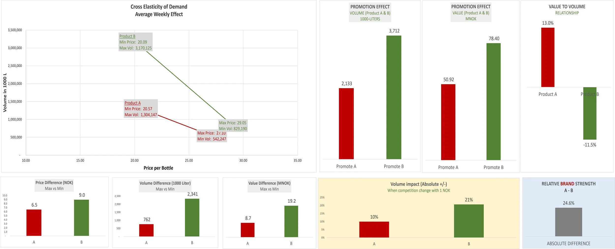
The yellow colored ‘area’ tells us that Product B is more sensitive to price changes than Product A. When A changes their price point with NOK 1, the sales of Product B changes with 21%. That means, that if A lowers the price point with NOK 1, the sales of Product B lowers with 21%, and vice versa. From the core graph, you can easily see that B is more elastic due to the steeper slope. If Product B changes their price with NOK 1, the sales of Product A changes with 10%. You might think that 10% vs 21% isn’t that big of a deal, but in absolute terms, a small price change for A affects the weekly sales of B by 4.25 times (A: 84,7 vs B: 360.2). Yes, B rocks the podium today, but depends on low prices and aggressive promotional presence to remain on top. Product A on the other side might seems to have everything right for a brighter future, where smartness and patience are key elements for success.
The question is what the two players should do? A destructive spiral where they go head to head and compete on the same pack and price points are not ideal to neither the two suppliers, nor the trade as a whole. Product A needs to be the smartest, as Product B leads the race, and sets the scene for action.
What should Product A do?
Product A needs to avoid a ‘tit for tat’ approach, and use smartness instead of biceps. It is easier said than done, but patience is a virtue for Product A, and will pay off in the longer run. Since B is more dependent on bigger packs and promotions, Product A should consider to up-size their single pack, and keep the same price point as Product B. This as a dual sided ‘value added’ approach. This way, the retailers can shift some of the promotional volume to single packs, and thereby improve the mix during weekdays. In addition, Product A should ideally take one account, and make that one a success story, by trying out various pack options for promotions; but not on the terms of Product B. Product A should be the value creator, and thereby best buddies of the retailers.
What should Product B do?
Product B’s role is to create foot traffic to the stores, and can thereby improve overall sales for the retailers. Product B should then consider to up-size their volume for promotions. They will then create excitement, remain their price leadership, as well as build in-home preference for Product B. Shoppers would thereby need to buy more to gain the benefits. If they do not want to buy a bigger volume pack, the shoppers can always take the smaller EDLP pack, still at favorable terms. This as a tool for Mix Management improvements, and long term brand building values. Down the road, some of the volume will shift to singles, and will thereby improve the overall mix.
With this in mind, we move over to the last stop in the Pricing Tool (Brand Strength Model), to measure pricing as a tool to understand brand strength over time. It is indeed powerful, as it also shows the potential for the brand owner and for the retailers to ignite exponential- and sustainable growth.